Consider a researcher wants to ascertain the extent to which individuals engage in various peculiar behaviors. Individuals are asked to estimate the extent to which they listen to Rolf Harris, discuss brands of nail clippers, enjoy statistics, store ear wax, examine gunk under toe nails, display their double jointed arms, ring people at 3.00 am, go home when it is their turn to shout drinks, and play music at maximum volume. An extract of the data is presented below (see Introduction to AMOS for more details).
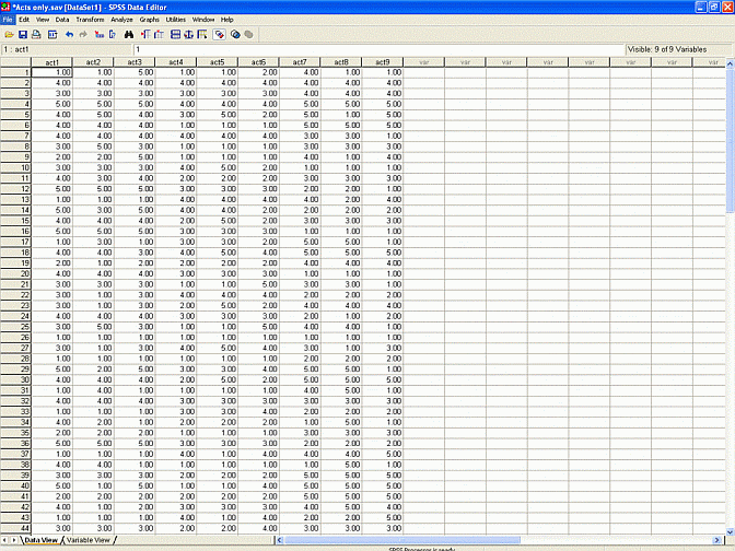
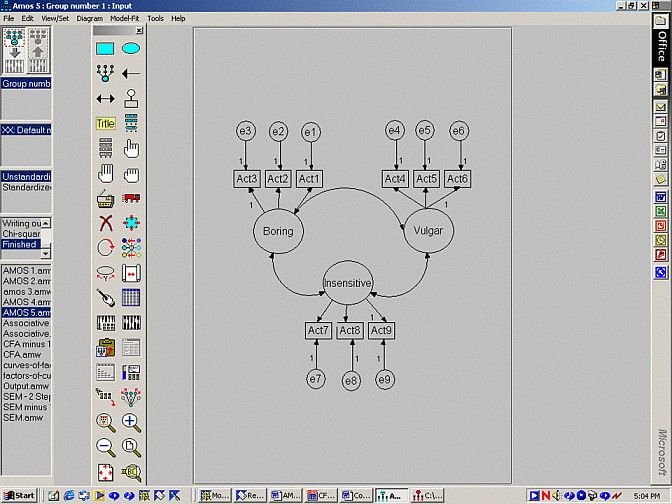
In addition, suppose these responses were subjected to an exploratory factor analysis. This analysis revealed the acts correspond to three distinct factors or clusters. Acts 1 to 3--listening to Rolf Harris, discussing brands of nail clippers, and enjoying statistics--represented one factor, which was labelled 'boring'. Acts 4 to 6--storing ear wax, examining gunk under toe nails, and displaying double jointed arms--represented the second factor, which was labelled 'vulgar'. Finally, Acts 7 to 9--ringing people at 3.00 am, going home when it is their turn to shout drinks, and playing music at maximum volume--represented the final factor, which was labelled 'insensitive'.
Unfortunately, these data were extracted from only one sample of University students. The same set of factors might not emerge from another sample of University students. Furthermore, the same set of factors might not emerge from a sample that does not comprise University students. In other words, these factors might reflect some peculiarity in the sample that was utilised. For example, another sample might reveal four distinct factors. Another sample might reveal that listening to Rolf Harris and storing ear wax pertain to the same factor, and so forth. To resolve this issue, the same questionnaire was administered to a broad sample of Australian employees. An extract of these data is presented below.
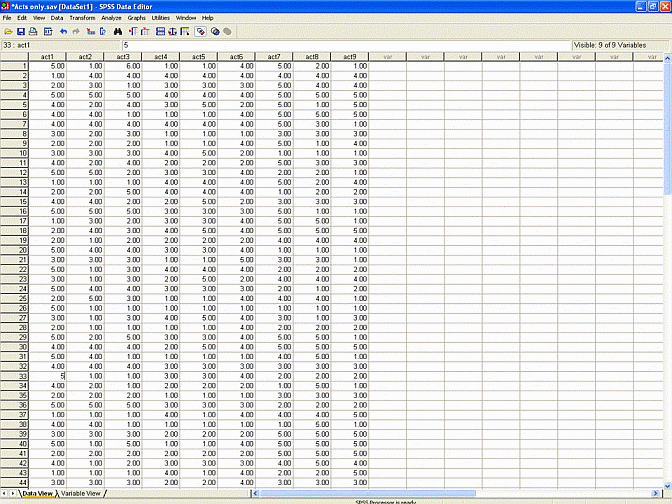
To ascertain whether or not these data yield the same three factors, another exploratory factor analysis can be applied. That is, these data can be subjected to an exploratory factor analysis - perhaps principal axis factoring with varimax rotation. The rotated matrix that emerges from this analysis appears in the table below.
| Peculiary acts | Factor 1 | Factor 2 | Factor 3 | |||
| Act 1 | 0.87 | 0.11 | 0.23 | |||
| Act 2 | 0.79 | 0.16 | 0.08 | |||
| Act 3 | 0.56 | 0.55 | 0.09 | |||
| Act 4 | 0.10 | 0.87 | 0.12 | |||
| Act 5 | 0.16 | 0.89 | 0.10 | |||
| Act 6 | 0.03 | 0.77 | 0.09 | |||
| Act 7 | 0.29 | 0.10 | 0.89 | |||
| Act 8 | 0.12 | 0.02 | 0.88 | |||
| Act 9 | 0.11 | 0.26 | 0.80 | |||
This output yields similar factors to the findings that were derived from the previous study. That is, Acts 1, 2, and perhaps 3 represent one factor. Acts 4, 5, 6, and perhaps 3 represent a second factor. Finally, Acts 7, 8, and 9 represent a third factor.
In other words, the only discrepancy between this output and the previous set of findings revolves around Act 3. That is, Act 3 seems to pertain marginally to more than one factor. But, this discrepancy might reflect random error. That is, this discrepancy might evaporate if the same individuals were retested. Factor analysis does not indicate whether or not this discrepancy is significant or legitimate.
Indeed, such discrepancies are almost inevitable. That is, the precise values are sensitive to minor factors and thus vary dramatically across samples. As a consequence, exploratory factor analysis should not be utilised to substantiate or validate a particular set of factors. That is, even random, trivial fluctuations in the data can generate findings that discredit the purported set of factors.
So, instead, another technique needs to be applied to substantiate or evaluate a hypothesised set of factors. That is, another technique needs to conducted to assess whether or not the data yield an expected set of factors. Confirmatory factor analysis affords a suitable means to assess these factors. In other words, confirmatory factor analysis can be utilised to assess whether or not the acts pertain to the hypothesised clusters.
To conduct this confirmatory factor analysis, the researcher needs to:
Regression weights
| . | Estimate | SE | CR | |||
| Act1 <--- boring | 0.8 | 0.2 | 4.0 | |||
| Act2 <--- boring | 1.2 | 3.5 | 3.5 | |||
| Act3 <--- boring | 1.0 | . | . | |||
| Act4 <--- vulgar | 0.9 | 0.2 | 4.5 | |||
| Act5 <--- vulgar | 0.6 | 0.3 | 3.0 | |||
| Act6 <--- vulgar | 1.0 | . | . | |||
| Act7 <--- insensitive | 1.5 | 1.5 | 1.0 | |||
| Act8 <--- insensitive | 0.8 | 0.2 | 4.0 | |||
| Act9 <--- insensitive | 1.0 | . | . | |||
This table is not especially informative. The important data appears in the column labelled CR. CR denotes 'Critical Ratio', which is equivalent to the regression weight divided by the standard error of this weight. The distribution of this ratio resembles a z distribution. As a consequence:
Second, the data in the column labelled 'Regression weights' can be used to create equations that relate each act to each factor. These equations are not especially useful, but can facilitate an understanding of confirmatory factor analysis. Specifically, these weights yield the following equations:
Act1 = 0.8 x Boring + error 1
Act2 = 1.2 x Boring + error 2 Act3 = 1.0 x Boring + error 3 Act4 = 0.9 x Vulgar + error 4 Act5 = 0.6 x Vulgar + error 5 Act6 = 1.0 x Vulgar + error 6 Act7 = 1.5 x Insensitive + error 7 Act8 = 0.8 x Insensitive + error 8 Act9 = 1.0 x Insensitive + error 9For example, according to the first equation:
The regression weights associated with Acts 3, 6, and 9 all equal 1. These weights are not coincidental. Instead, you might recall, the diagram had already set these regression weights to 1. As a consequence, AMOS did not attempt to estimate the weights associated with these items, but instead assumed they equalled 1.
To appreciate who these regression weights were set to 1:
Second, locate the table that is titled 'Standardised Regression weights'. This table presents the regression weights that would have emerged had the measured variables first been converted to z scores - by deducting the mean and dividing by the standard deviation.
Standardised Weights
| . | Estimate | |||||
| Act1 <--- boring | 0.7 | |||||
| Act2 <--- boring | 1.0 | |||||
| Act3 <--- boring | 0.8 | |||||
| Act4 <--- vulgar | 0.7 | |||||
| Act5 <--- vulgar | 0.8 | |||||
| Act6 <--- vulgar | 0.8 | |||||
| Act7 <--- insensitive | 0.9 | |||||
| Act8 <--- insensitive | 0.6 | |||||
| Act9 <--- insensitive | 0.8 | |||||
Of course, researchers seldom, if ever, convert all the measured variables to z scores. At first glance, therefore, this output might not seem especially informative. However, the magnitude of these values can be used to identify variables that are not closely related to the corresponding factors. Regression weights below 0.5 or so indicate variables that are not especially aligned with the factors.
You should next locate the table entitled 'Covariances'. Again, only the CR column is informative. CR values above 2 indicate the corresponding pair of factors significantly covary;& in other words, these factors are correlated. CR values less than 2 indicate the corresponding pair of factors do not covary;& in other words, they are not related.
Covariances
| . | Estimate | SE | CR | |||
| boring <---> vulgar | 0.9 | 0.2 4.0 | ||||
| boring <---> insensitive | 1.2 | 3.5 3.5 | ||||
| insensitive <---> boring | 1.0 | 0.1 10.0 | ||||
The values in the column labelled 'Estimate' are less informative. They represent the covariance between the corresponding factors. Covariance mirrors correlation, but does not vary from 1 to -1. Hence, the magnitude of these numbers is not informative. Instead, users should consult the following table, which presents the correlation between each pair of factors.
Correlation
| . | Estimate | |||||
| boring <---> vulgar | 0.2 | |||||
| boring <---> insensitive | 0.5 | |||||
| insensitive <---> boring | 0.3 | |||||
Fortunately, AMOS provides a series of indices that can be utilised to assess whether or not the data conform to the hypothesised model. In other words, these indices reflect the extent to which the variables correlate with one another as the model would predict. A subset of these indices is presented below.
__
Chi-square = 25.534 Degrees of freedom = 24| Model | NPAR | CMIN | DF | P | CMIN/DF | |
| Default model | 21 | 21.72 | 24 | 0.596 | 0.905 | |
| Saturated model | 45 | 0 | 0 | . | . | |
| Independence | 9 | 51.99 | 36 | 0.041 | 1.44 | |
| Zero model | 0 | 220.5 | 45 | 0.00 | 4.90 | |
| Model | RMR | GFI | AGFI | PGFI | ||
| Default model | 0.163 | 0.901 | 0.81 | 0.481 | ||
| Saturated model | 0 | 1.00 | . | . | ||
| Independence | 0.523 | 0.76 | 0.71 | 0.611 | ||
| Zero model | 0.761 | 0.00 | 0.00 | 0.00 | ||
| Model | NFI | RFI | IFI | TLI | CFI | |
| Default model | 0.667 | 0.388 | 0.667 | 0.388 | 0.667 | |
| Saturated model | 1.00 | . | 1.00 | . | 1.00 | |
| Independence | 1.00 | 0.00 | 0.00 | 0.00 | 0.00 | |
| Model | RMSEA | LO 90 | HI 90 | PCLOSE | ||
| Default model | 0.00 | 0.00 | 0.103 | 0.735 | ||
| Independence | 0.09 | 0.02 | 0.149 | 0.116 | ||
| Model | AIC | BCC | BIC | CAIC | ||
| Default model | 63.7 | 74.49 | 150.0 | 124.8 | ||
| Saturated model | 90.0 | 113.1 | 274.9 | 221.0 | ||
| Independence | 69.93 | 74.68 | 110.0 | 96.20 | ||
| Zero model | 220 | 220.5 | 220.5 | 220.5 | ||
Probability level = 0.377
At first glance, these indices might seem overwhelming. Indeed, AMOS actually presents several additional tables of indices. In practice, however, these indices can be interpreted readily. In particular:
o The p value associated with the chi-square should exceed 0.05
o CMIN/DF, which is the chi-square divided by the df value, should ideally be less than 2.0
o RMSEA, which denotes root mean square of the residuals, should be less than 0.05
o GFI, AGFI, NFI, and CFI should exceed 0.9.
o Different journals do not all emphasise the same indices. One journal might demand that researchers report GFI and AGFI, whereas another journal might not demand that researchers report these indices. Always check previous articles in the target journal.
Three possible outcomes can arise. First, the fit indices can generally indicate the model is ascurate. In other words, the p value exceeds 0.05, the root mean square error is less than 0.05, NFI exceeds 0.9, and so on. This outcome would confirm the hypothesised model.
Second, the fit indices might indicate the model is inaccurate. In other words, the p value is less than 0.05, the root mean square error exceeds 0.05, NFI is less than 0.9, and so forth. This outcome would suggest the hypothesised model is unsuitable. For example:
In other words, items that pertain to the same factor might not correlate with each other to the same degree. Alternatively, items that pertain to separate factors might correlate with each other excessively.
Several limitations in the data could yield these errors. The most common limitation revolves around an issue called identification. Sometimes, the output is designated as under-identified. This term suggests that insufficient information is provided to estimate the coefficients or compute the indices. To ensure that sufficient information is available in the data, two conditions must be satisfied.
First, the degrees of freedom, which AMOS specifies in the output, must exceed 0. Strictly speaking, the degrees of freedom equals the number of informative terms minus the number of coefficients to be estimated. In practice, the number of informative terms usually equals the number of items x the number of items - 1. The number of estimations usually equals the number of arrows without numbers or ovals without variances. The df will tend to exceed 0 provided the model comprises at least 3 items per factor.
Second, severe multi-colinearity must be eradicated. That is, no pair of items should be too highly correlated with one another. For example, Acts 1 and 2 should not be too highly correlated with each other. Correlations that exceed 0.9 or so for example could induce under-identification. That is, the items become too correlated to distinguish. Thus, these correlated items effectively do not confer distinct information.
To appreciate this rationale, consider the following equations:
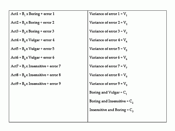
The equations on the left-hand side link each measured variable to a specific factor. The equations on the right-hand side represent the variance of each error and the correlation between each pair of factors. B1 to B9 represent regression weights or numbers. V1 to V9 represent the variance of each error. C1 to C3 represent correlations between each pair of factors.
In essence, the role of AMOS is to estimate these parameters - that is, B1 to B9 , V1 to V9 , and C1 to C3. That is, AMOS attempts to determine the values that seem most consistent with the data. The question, then, becomes how does AMOS estimate these parameters or values? Roughly speaking, AMOS first utilises some crude, inaccurate algorithm or formula to estimate these values or parameters. These initial values are presented below.
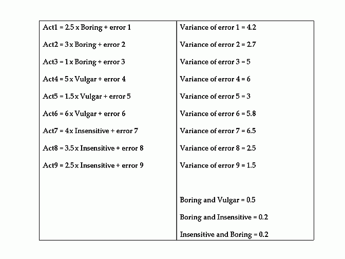
AMOS then determines the extent to which the data seems to conform to these equations. Specifically, using formulas that will be discussed later, AMOS computes the extent to which the data depart from the pattern these equations would predict. That is, AMOS calculates a discrepancy score, such as "Discrepancy = 3.5"
AMOS uses other algorithms and formulas that adjust these values or parameters to reduce this discrepancy. For instance, the second attempt to estimate these values is presented below.
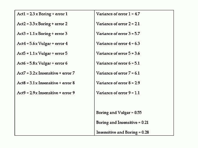
This process continues until the discrepancy hardly improves at all. Nevertheless, sometimes this process uncovers implausible values by chance. For instance, this process might estimate the variance of error 1 equals -0.5 - an impossible value. Alternatively, this process might estimate the correlation between two factors is 1.5 - another impossible value. At this point, AMOS ceases the process and reports an error.
This problem does not reflect a shortfall in the data. Instead, this problem merely reflects a misfortune. Indeed, had AMOS selected different initial values or parameters, this difficulty might not have arisen. Unfortunately, AMOS is not programmed to select different initial values. Instead, the researcher has to specify different initial values. That is, the researcher can specify the values that AMOS should apply to the first set of equations.
To specify these initial values:
First, researchers can estimate the values that participants would have generated on these missing data points. Specifically, they should:
When you execute AMOS, the same problem will arise again. This problem arises again because AMOS uses the original data until the program is deactivated. Therefore, you need to:
Second, another technique can be used to accommodate missing data. In particular, AMOS can accept missing data after the researcher:
This practice, however, does present some minor drawbacks. First, when the option 'Estimate intercepts and means' is selected, AMOS undertakes a more comprehensive and informative process. Specifically, AMOS estimates the mean of some factors and the intercept of others - a distinction that does not need to be understood at this stage. This process influences the df, goodness-of-fit indices, and other facets of the output. As a consequence, this process could diminish the goodness-of-fit.
Second, maximum likelihood presents some minor drawbacks as well. These drawbacks are outlined in the next section.
First, after each set of equations is formulated, AMOS computes the covariance matrix this model would predict. A covariance is tantamount to a correlation. Strictly speaking, a covariance is the correlation multiplied by the standard deviation of each variable. An extract of this covariance matrix is presented below.
| . | Act 1 | Act 2 | Act 3 | ... | ||
| Act 1 | 4.6 | . | . | ... | ||
| Act 2 | 1.7 | 6.4 | . | ... | ||
| Act 3 | 4.8 | 7.3 | 2.5 | ... | ||
| ... | ... | ... | ... | ... | ||
Second, AMOS computes the covariance matrix from the dataset - in other words, the actual or observed covariance matrix. An extract is presented below.
| . | Act 1 | Act 2 | Act 3 | ... | ||
| Act 1 | 3.9 | . | . | ... | ||
| Act 2 | 2.5 | 7.4 | . | ... | ||
| Act 3 | 9.8 | 2.3 | 1.3 | ... | ||
| ... | ... | ... | ... | ... | ||
Third, the discrepancy between these matrices is computed. The formula that is utilised to compute these discrepancies depends on the estimation method. For example, according to unweighted least squares, the difference between each corresponding cell in the two matrices is computed and these differences are then summed. As an aside, chi-square is simply this discrepancy value multiplied by the sample size. To illustrate, in the previous example, the discrepancy is...
Discrepancy = |4.6 - 3.9| + |1.7 - 2.5| + |6.4 - 7.4| + |4.8 - 9.8| ...
The formula is similar, but adjusted marginally, when maximum likelihood is utilised. Specifically, AMOS again determines the difference between each corresponding cell in the two matrices. AMOS then divides each difference by the corresponding covariance in the model matrix. An illustration is presented below.
Discrepancy = |4.6 - 3.9|/4.6 + |1.7 - 2.5|/1.7 + |6.4 - 7.4|/6.4 + |4.8 - 9.8|/4.8 ...
Likewise, the formula is similar when generalised least squares is selected. Again, AMOS first determines the difference between each corresponding cell in the two matrices. AMOS then divides each difference by the corresponding covariance in the data matrix. An illustration is presented below.
Discrepancy = |4.6 - 3.9|/3.9 + |1.7 - 2.5|/2.5 + |6.4 - 7.4|/7.4 + |4.8 - 9.8|/9.8 ...Finally, the formula is similar, but more complex, when arbitrary distribution free is applied. As usual, AMOS first determines the difference between the corresponding covariances. AMOS then divides each difference by some term that represents the kurtosis of each variable;& the precise algorithm, however, is beyond the scope of this document. An illustration is presented below.
Discrepancy = |4.6 - 3.9|/2.3 + |1.7 - 2.5|/5.9 + |6.4 - 7.4|/4.6 + |4.8 - 9.8|/5.1 ...
The obvious question, then, becomes which of these techniques are most applicable. The following principles need to be considered.
In short, maximum likelihood is perhaps the most common method to apply;& arbitrary distribution free is suitable only if the sample size is particularly large.
To reiterate, arbitrary distribution free is the only estimation technique that is applicable when the data do not conform to a multivariate normal distribution. Unfortunately, this technique is not suitable unless the sample size is especially extensive. Specifically, if the sample size is less than 2500 or so, maximum likelihood or generalised least squares needs to be applied. Hence, the data should demonstrate multivariate normality.
To ensure the data conform to this distribution, the researcher should first identify and delete multivariate outliers. AMOS provides some options that can be utilised to uncover these outliers. Specifically, the researcher should:When the model is executed, AMOS will specify the probability that each individual differs significantly from everyone else. An extract of this table is presented below. p1 values less than 0.001 might indicate a multivariate outlier. Hence, the corresponding individuals might need to be excluded.
| Observation number | Mahalanobis d squared | P1 | P2 | |||
| 3 | 35.7 | 0.054 | 0.985 | |||
| 87 | 31.6 | 0.086 | 0.953 | |||
| 105 | 29.8 | 0.103 | 0.835 | |||
| . | . | . | . | |||
| . | . | . | . | |||
| 16 | 1.4 | 0.967 | 0.014 | |||
Once these outliers are removed, the researcher should then assess whether or not the assumption of multivariate normality has been fulfilled. Specifically, AMOS presents a table that represents the skewness and kurtosis of each variable as well as a test of multivariate normality. An extract of this table is presented below.
| . | min | max | skew | CR | kurtosis | CR |
| Act 1 | 1 | 5 | 2.5 | 1.3 | 4.5 | 1.2 |
| Act 2 | 1 | 5 | 1.5 | 0.8 | 5.6 | 1.8 |
| Act3 | 1 | 5 | 1.7 | 1.2 | 7.6 | 2.1 |
| . | . | . | . | . | . | . |
| . | . | . | . | . | . | . |
| Multivariate | . | . | . | . | 6.5 | 2.4 |
The first CR column can be utilised to ascertain whether or not the corresponding skewness is significant. The second CR column can be utilised to ascertain whether or not the corresponding kurtosis is significant. For example, the kurtosis associated with Act 3 equals 7.6 and the corresponding CR value exceeds 2. In other words, the kurtosis of Act 3 significantly exceeds 0 and thus is not normal. Nevertheless, skewness values that are less than 2 or kurtosis values that are less than 5 do not undermine the output appreciably. Hence, Act 3 can be included.
The final row assesses the assumption of multivariate normality. If the CR value is less than 2, the assumption of multivariate normality can be deemed as fulfilled. If this assumption is not fulfilled, some of the variables might need to be removed or transformed.
Sometimes, all the assumptions and requirements are fulfilled - the model is over-identified, multicolinearity is absent, the assumptions are fulfilled, and the sample size is large - but the goodness-of-fit indices still indicate the model is inconsistent with the data. This finding suggests the model might need to be refined. For example:
Fortunately, AMOS can provide some information that can be utilised to determine how the model should be refined. Specifically, before the model is executed, the researcher should:
| Covariances | MI | Par Change | ||||
| Error1 <---> Error4 | 15.6 | 0.324 | ||||
| Error4 <---> Error6 | 11.5 | 0.313 | ||||
| Error 4 <---> Error8 | 10.5 | 0.143 | ||||
| Variances | MI | Par Change | ||||
| . | . | . | ||||
| Regression weights | MI | Par Change | ||||
| Act4 <---> Act1 | 10.6 | 0.23 | ||||
| Act5 <---> Act3 | 11.4 | 0.15 | ||||
These tables can be used to identify discrepancies from the hypothesised model. To appreciate this table, consider the first row, which indicates the modification index associated with Error1 <---> Error4 is 15.6. This finding indicates that:
The researcher should continue these refinements, until the goodness-of-fit indices indicate the model is applicable. These refinements could include discarding measured variables, permitting correlations between factors that had been assumed to be independent, or even adding additional factors.
Confirmatory factor analysis can be utilized to control various forms of variance. For example, as Le, Schmidt, Harter, and Lauver (2010) showed, because some forms of variance are disregarded, individuals often underestimate the overlap between two scales, overlooking possible redundancies. To illustrate, Le, Schmidt, Harter, and Lauver (2010) distinguished five sources of variance in measures, such as job satisfaction:
According to Le, Schmidt, Harter, and Lauver (2010), because many sources of variance affect responses, researchers often underestimate the association between constructs. To illustrate, research indicates that job satisfaction and organizational commitment are highly associated with each other, but nevertheless distinct. Correlations might approach about .70.
Because the correlation is appreciably less than 1, researchers will maintain that job satisfaction and organizational commitment are distinct. Nevertheless, the true scores on these scales might be identical, and hence the measures might be redundant. That is, the correlation might not be 1 merely because random response error, item specific error, transient error, and factor specific error contaminated the responses.
Admittedly, researchers do sometimes include formulas that are intended to estimate, and then discount, two sources of variance: random response error and item specific error. Traditional forms of attenuation nullify these sources of error. However, these corrections do not override transient error or factor specific error. To illustrate the problem with factor specific error, for example, two measures of job satisfaction might be as distinct from each other as a measure of job satisfaction and a measure of organizational commitment.
To override this problem, in one study, conducted by Le, Schmidt, Harter, and Lauver (2010), participants completed two measure of job satisfaction and two measures of organizational commitment at two times. They also completed measures of positive and negativity affectivity. Responses were subjected to confirmatory factor analysis to control the various sources of error. For example, each of the measures, at each time, were assumed to be influenced by three latent constructs: the overall construct, such as job satisfaction, a time specific construct, such as job satisfaction at Time 1, and a measure specific construct, such as the first measure of job satisfaction.
When this approach was utilized, the association between the true scores of job satisfaction and the true scores of organizational commitment was especially high, at .91--almost indicating these concepts are redundant, despite their conceptual differences. Furthermore, these true scores of job satisfaction and organizational commitment were related to positive and negative affectivity to the same extent. That is, the nomological networds seemed the same: They were associated with other measures to the same degree and thus could not be differentiated empirically.
Le, H., Schmidt, F. L., Harter, J. K., & Lauver, K. J. (2010). The problem of empirical redundancy of constructs in organizational research: An empirical investigation. Organizational Behavior and Human Decision Processes, 112, 112-125.
Last Update: 6/2/2016