This article assumes knowledge that was presented in the documents entitled Introduction to AMOS and Confirmatory factor analysis.During these document, confirmatory factor analysis was undertaken toassess whether or not a series of annoying acts correlate with oneanother as anticipated. In other words, this analysis was conducted toascertain whether or not the various items pertain to the hypothesizedfactors. The following table presents an extract of these data.

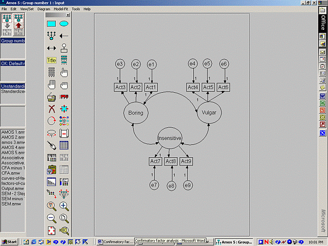
To ascertain whether or not the items pertain to the hypothesisedfactors, a diagram that represents the hypothesised model was createdand then evaluated using AMOS. This model is presented below. Thismodel indicates that Acts 1 to 3 pertain to one factor. Acts 4 to 6pertain to another factor. Finally, Acts 7 to 9 pertain to a thirdfactor. All of these factors are assumed to be correlated with oneanother.

An extract of the output is presented below. This output suggests thecorrelation between boring and vulgar is 0.2. The CR value thatcoincides with this correlation or covariance exceeds 2 and thus can beregarded as significant. Likewise, the CR values that coincide with theother correlations or covariances exceed 2 and can thus be regarded assignificant as well. In other words, this model suggests the factorsare correlated
Covariances
| . | Estimate | ...SE... | ...CR... | |||
| boring <---> vulgar | 0.9 | 0.2 | 4.0 | |||
| boring <---> insensitive | 1.2 | 3.5 | 3.5 | |||
| insensitive <---> boring | 1.0 | 0.1 | 10.0 | |||
Correlation
| . | Estimate | |||||
| boring <---> vulgar | 0.2 | |||||
| boring <---> insensitive | 0.5 | |||||
| insensitive <---> boring | 0.3 | |||||
To reiterate, the previous analysis indicated the factors--boring,vulgar, and insensitive--are correlated with each other. This output,however, does not uncover the causal network that links these factors.For example, perhaps levels of both vulgar and insensitive influencelevel of boring. That is,
Structural equation modelling (SEM) can be applied to examine theserelationships. That is, SEM can be conceptualised as an extension ofconfirmatory factor analysis. Like confirmatory factor analysis, SEMdetermines whether or not the items pertain to the hypothesisedfactors. However, SEM also explores the relationships between thesefactors. In contrast, confirmatory factor analysis can merely ascertainwhether or not these factors are correlated
In short, SEM assesses the relationships that link the various factors.This function of SEM imparts important information. Specifically, SEMcan be applied to differentiate direct and indirect relationships. Toillustrate, consider the following series of equations.
According to these relationships:
In other words, if the level to which individuals are insensitive issomehow controlled, increases in vulgarity will not determine theextent to which they are boring. In statistical parlance, insensitivitymediates the relationship between vulgar and boring. As a consequence,structural equation modelling can be applied to establish mediation.
The previous section revealed that SEM confers benefits thatconfirmatory factor analysis cannot provide. Specifically, SEM canuncover mediators. Nevertheless, multiple regression can also servethis function. To illustrate, consider the table below. These columnsrepresent the average of each set of items. That is, the first columnrepresents the average response to Acts 1 to 3 of each participant. Forexample, the first participant specified '5' in relation to Act 1, '1'in relation to Act 2, and '2' in relation to Act 3. The average of 5,1, and 2 is 2.67. Hence, this column effectively denotes the scores onthe first factor: boring.
| Factor 1 | Factor 2 | Factor 3 | ||||
| 2.67 | 1.67 | 2.33 | ||||
| 2.33 | 3.33 | 3.33 | ||||
| 3.67 | 2.67 | 3.33 | ||||
| 3.00 | 3.00 | 3.67 | ||||
| 3.00 | 3.00 | 2.67 | ||||
| 3.00 | 2.67 | 2.67 | ||||
| 4.00 | 4.00 | 2.33 | ||||
| . | . | . | ||||
| . | . | . | ||||
| 2.33 | 3.33 | 3.33 | ||||
The second column represents the average response to Acts 4 to 6 andthus denotes the scores on the second factor: vulgar. The final columnrepresents the average response to Acts 7 to 9 and thus denotes scoreson the third factor: insensitive. These averages can then be subjectedto multiple regression. For example, suppose the researcher needed tosubstantiate the following relationships:
To assess the first equation through multiple regression:
To assess the second equation:
Furthermore, to verify that vulgar is not directly related to boring, another equation would be explored. Specifically:
In short, a series of regression equations can also differentiatedirect and indirect relationships and thus establish mediation.Nevertheless, structural equation modelling presents several benefitsover multiple regression.
First, structural equation modelling can unearth items that pertain toseparate factors but overlap inordinately. For example, recall thatActs 1 pertains to the boring factor and Act 7 pertains to theinsensitive factor. Nevertheless, the researcher might have overlookedthe observation that Acts 1 and 7 are similar.
Now suppose the researcher subjects these factors to multipleregression. These analyses would reveal that boring and insensitive arehighly correlated. Unfortunately, this correlation could merely reflectthe artificial and unintended overlap between Acts 1 and 7. The otheritems that pertain to boring might not correlate with the other itemsthat pertain to insensitive. In other words, the observed correlationbetween boring and sensitive might reflect an error in the variablesthat were selected to represent each factor.
SEM, however, precludes this complication. SEM would uncover theoverlap between Acts 1 and 7. Specifically, this elevated correlationwould compromise the fit indices. Hence, the researcher would probablydetect and thus eliminate the inflated correlation between Acts 1 and 7.
Second, some forms of SEM are less sensitive to violations ofnormality. That is, multiple regression is contaminated if thedistribution of errors severely departs from normality. In contrast,SEM is not contaminated by these departures, provided the method calledarbitrary distribution free is applied. Unfortunately, this method canbe applied only if the sample size is particularly large, ideally morethan 1000.
Finally, SEM does provide several other minor benefits. For example,SEM analyses the error terms, which provides additional information andenhances power. In addition, SEM presents many fit indices, which canbe used to ascertain which variables should be included.
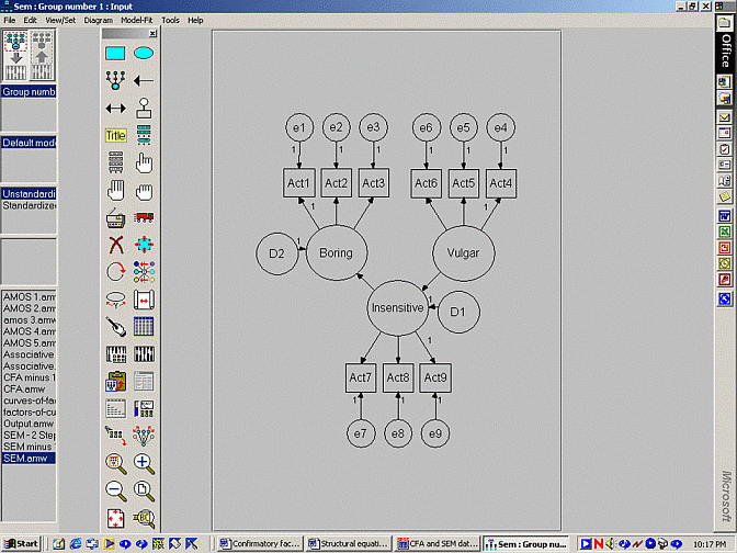
The procedure that is utilised to conduct confirmatory factor analysisis almost identical to the process that needs to be followed toundertake SEM. That is, the user merely needs to construct a diagramand then analyse the model. A typical diagram is presented below.

The process that needs to be followed is identical to confirmatoryfactor analysis, apart from the following disparities. First, thedouble-headed arrows that link the factors are replaced withsingle-headed arrows. For example, according to this model, boring is afunction of insensitive and insensitive is a function of vulgar.
Second, error terms have to be added to all the factors that intersectwith the head of an arrow. In this model, error terms have to beappended to both boring and insensitive. The error terms are oftenlabelled as 'D' to denote 'disturbance'. To appreciate the function ofthese error terms, recall the equations that link the factors:
Third, the output presents marginally different information.Specifically, the output does not reveal the correlation or covariancebetween the factors. Instead, the output presents the regressionweights that pertain to each relationship. An example is displayedbelow.
Regression weights
| . | Estimate | ...SE... | ...CR... | |||
| Insensitive <--- Vulgar | 0.8 | 0.2 | 4.0 | |||
| Boring <--- Insensitive | 1.3 | 3.5 | 3.5 | |||
| Act1 <--- boring | 0.9 | 0.2 | 4.0 | |||
| Act2 <--- boring | 1.2 | 3.5 | 3.5 | |||
| Act3 <--- boring | 1.0 | . | . | |||
| Act4 <--- vulgar | 0.9 | 0.2 | 4.5 | |||
| Act5 <--- vulgar | 0.6 | 0.3 | 3.0 | |||
| Act6 <--- vulgar | 1.0 | . | . | |||
| Act7 <--- insensitive | 1.5 | 1.5 | 1.0 | |||
| Act8 <--- insensitive | 0.8 | 0.2 | 4.0 | |||
| Act9 <--- insensitive | 1.0 | . | . | |||
As indicated in the top two rows of this table:
The previous section revealed that regression weights that relate thefactors reached significance. These conclusions, however, assume the CRvalues conform to a z distribution. Strictly speaking, this assumptionis upheld only when the sample size is extremely large. When the sampleis less than 1000, for example, another method should be utilised toassess whether or not each regression weight is significant.
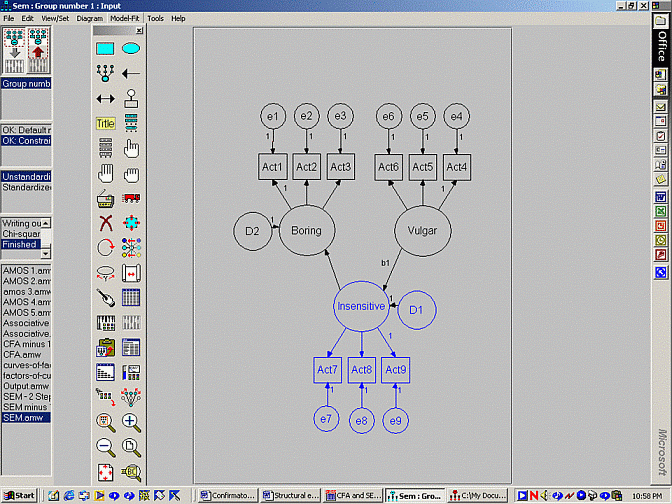
Fortunately, another method - called nested models - has been createdto assess specific regression weights. The rationale conforms to thefollowing logic:
To undertake this process:

Second model
| DF | CMIN | p | NFI Delta 1 | IFI Delta 2 | Rho 1 | Rho 1 |
| 1 | 3.977 | 0.040 | 0.014 | 0.015 | -0.011 | -0.016 |
This output suggests the difference in chi-square values between thesemodels is 3.977, as specified in the column CMIN. The p valueassociated with this difference is 0.04, which is less than 0.05 oralpha. Accordingly:
To reiterate, SEM fulfils two objectives. First, like confirmatoryfactor analysis, SEM investigates the relationships between measuredvariables and factors. This component is called the measurement model.Second, SEM investigates the relationships between the factorsthemselves. This component is called the structural model. In theprevious example, the measurement and structural models are assessessimultaneously.
Some researchers, however, prefer to separate the two analyses. Thatis, some researchers like to concentrate on the measurement model firstand subsequently focus on the structural model. Specifically, theseresearchers:
Regression weights
| . | Estimate | ...SE... | ...CR... | |||
| Act1 <--- boring | 0.9 | 0.2 | 4.0 | |||
| Act2 <--- boring | 1.2 | 3.5 | 3.5 | |||
| Act3 <--- boring | 1.0 | . | . | |||
| Act4 <--- vulgar | 0.9 | 0.2 | 4.5 | |||
| Act5 <--- vulgar | 0.6 | 0.3 | 3.0 | |||
| Act6 <--- vulgar | 1.0 | . | . | |||
| Act7 <--- insensitive | 1.5 | 1.5 | 1.0 | |||
| Act8 <--- insensitive | 0.8 | 0.2 | 4.0 | |||
| Act9 <--- insensitive | 1.0 | . | . | |||
Variances
| . | Estimate | ...SE... | ...CR... | |||
| Boring | 0.9 | 0.2 | 4.0 | |||
| Vulgar | 1.2 | 3.5 | 3.5 | |||
| Insensitive | 1.0 | 1.0 | 1.0 | |||
| Error 1 | 0.9 | 0.2 | 4.5 | |||
| Error 2 | 0.6 | 0.3 | 3.0 | |||
| Error 3 | 1.3 | 1.3 | 1.0 | |||
| Error 4 | 1.5 | 1.5 | 1.0 | |||
| Error 5 | 0.8 | 0.2 | 4.0 | |||
| Error 6 | 1.0 | 0.5 | 2.0 | |||
| Error 7 | 1.5 | 1.5 | 1.0 | |||
| Error 8 | 0.8 | 0.2 | 4.0 | |||
| Error 9 | 0.6 | 0.6 | 1.0 | |||
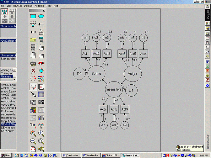
Then, researchers undertake the SEM, except apply these regression weights and variances to the model, as depicted below.

AMOS can also provide additional output. Specifically, using the iconthat appears below the magic wand and above the clipboard, you canrequest additional output, such as:
Last Update: 6/2/2016