MANOVAs or multivariate ANOVAs

Author: Dr Simon Moss

Introduction

ANOVAs are applied to compare groups, such as the two sexes, on one numerical variable, such as IQ, only. MANOVAs are used to compare groups on more than one numerical variable at the same time, such as IQ and wage. Sometimes, if the MANOVA generates significant effects, researchers then conduct subsequent ANOVAs to examine which variables differ across the groups.

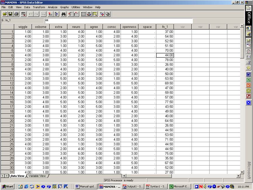
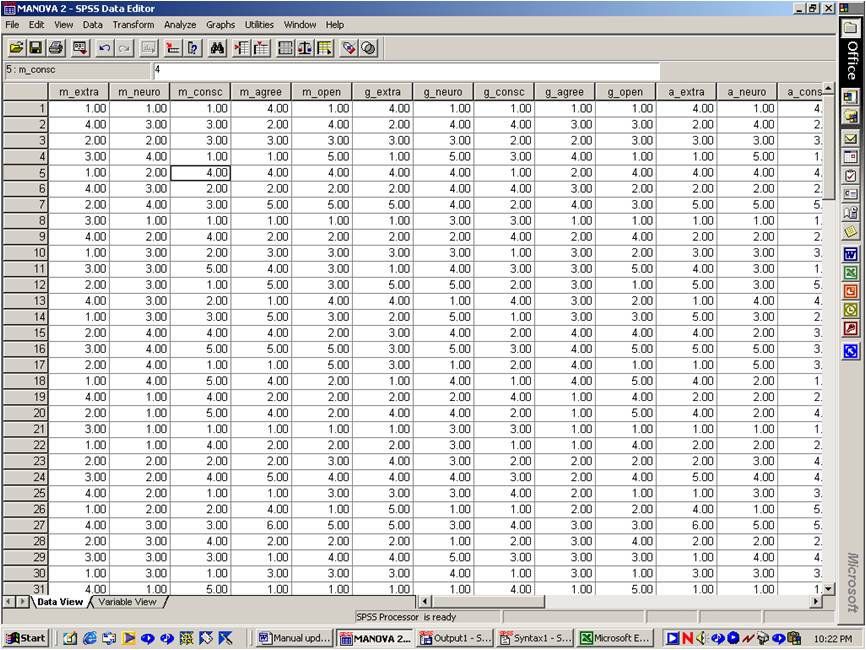
To illustrate, everyone prefers one Wiggle over the others. In addition, although they are difficult to differentiate, everyone prefers one Osborne over the others. Recently, a researcher decided to investigate whether or not the personality profile of individuals is dependent upon their favourite Wiggle or Osborne. Hence, 200 lecturers were asked to specify their favourite Wiggle--Murray, Sam, Anthony, or Jeff--and their favourite Osborne--Ozzy, Kelly, Sharon, and Jack. In addition, they completed the NEO to ascertain their level of extroversion, neuroticism, agreeableness, conscientiousness, and openness to experience. The following table presents an extract of the results.

Drawbacks of ANOVAs

To resolve this vexed issue, the researcher could undertake a series of 2-way ANOVAs, where favourite Wiggle and Osborne represent the two factors or independent variables. In particular:

• The first ANOVA could ascertain whether or not extroversion depends on favourite Wiggle and Osborne.
• The second ANOVA could ascertain whether or not neuroticism depends on favourite Wiggle and Osborne, and so forth.

In short, a series of five ANOVAs would need to be conducted. If any of these ANOVAs yield a Type I error--that is, an erroneous significant outcome--the researcher would conclude that favourite Wiggle or favourite Osborne does indeed coincide with personality. Because the researcher needs to undertake several analyses, the likelihood that one or more of these ANOVAs would yield a Type I error exceeds 0.05. In other words, the likelihood the researcher would erroneously claim that favourite Wiggle or favourite Osborne coincides with personality exceeds the accepted level of 0.05. Of course, this problem can be readily circumvented. In particular,

• The researcher can adjust the level of alpha from 0.05 to 0.01.
• That is, 0.05 can be divided by the number of analyses--a process that is usually called a Bonferroni adjustment.
• This adjustment, however, compromises the statistical power of these analyses.
• That is, genuine differences are more likely to be overlooked.

In contrast, MANOVA somehow combines all of the measures into a single column. This procedure then determines whether or not this single column depends on the factors, in this instance, favourite Wiggle and Osborne. Accordingly, MANOVA does not assess the same hypothesis on many separate occasions and thus circumvents the inflation of Type I errors without the need to adjust the level of alpha from 0.05 to 0.01.

Indeed, MANOVA incorporates another principle to optimise power. Specifically, this technique combines the measures using a formula that somehow maximises the difference between the groups. As a consequence, in some instances, a MANOVA can generate a significant finding even when the corresponding ANOVAs all yield nonsignificant outcomes. Specifically:

• The relative power of MANOVAs is especially apparent if the various measures--in this instance, extroversion, neuroticism, agreeableness, conscientiousness, and openness to experience--are moderately correlated with one another.
• In contrast, MANOVA is not especially powerful when the various measures are considerably or negligibly correlated with one another.

Step 1: Conduct the MANOVA

To implement a MANOVA when none of the factors are repeated measures, you need to complete the following steps:

1. Select "General Linear Model" and then "Multivariate" from the "Analyse" menu, after opening the relevant data file.
2. Specify the measures, such as personality measures, in the box labelled "Dependents".
3. Specify the independent variables, such as Wiggle and Osborne, in the box labelled "Fixed factors".
4. Press 'Options' and select "Homogeneity tests" from the Display options.
5. Press OK.

To interpret the outcomes, locate a table that is entitled "Multivariate tests". This table is presented below.

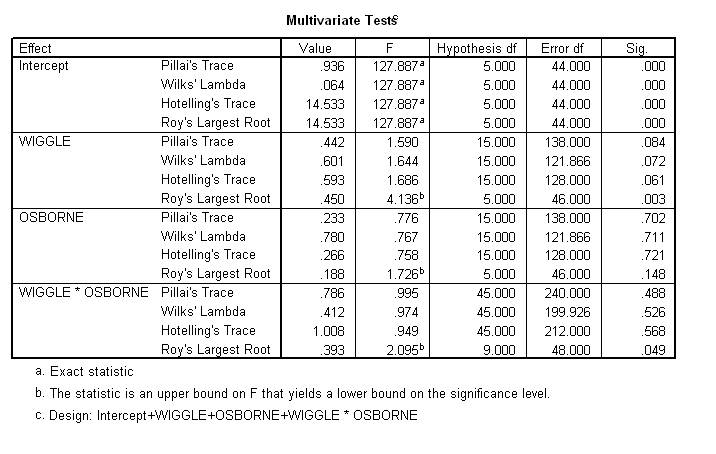
In this example, the researcher is interested in three outcomes: the effect of favourite Wiggle, the effect of favourite Osborne, and the interaction between favourite Wiggle and Osborne. To identify whether or not these effects are significant, the researcher should:

• Locate the row in the table that corresponds to the first factor, favourite Wiggle.
• Locate the column that corresponds to the p value, called 'Sig'.
• You will notice this row yields four p values.
• Most researchers utilise the p value that pertains to Pillais Trace.
• If this p value is less than 0.05, you can conclude the first factor, favourite Wiggle, is significantly related to the measures, personality.
• If this p value exceeds 0.05, you cannot conclude the first factor, favourite Wiggle, is significantly related to the measures, personality.

You can then apply the same process to the second factor, favourite Osborne, as well as the interaction. For example, if the p value that pertains to the interaction is less than 0.05, you can conclude the effect of favourite Wiggle on personality depends on favourite Osborne, and vice versa. In this instance, none of the effects attained significance according to the Pillai"s Trace.

Rationale behind one-way MANOVAs

The rationale behind MANOVA is complex. This rationale might become more comprehensible after you understand discriminant function analysis. To simplify this discussion, suppose instead the researcher discards favourite Osborne and thus undertakes a one-way MANOVA only. To ascertain the impact of the other factor, favourite Wiggle, SPSS computes an additional column that somehow integrates the five measures. For instance, the following formula might have been utilised to create this additional column:

Function 1 = 2.5 x Extroversion + 1.5 x Neuroticism + 4.0 x Conscientiousness + 5.0 x Agreeableness + 4.5 x Openness to Experience

This column, sometimes called a function, variate, or linear combination, is presented in the table below. In practice, this function does not appear in the SPSS datasheet, but is presented here merely to facilitate learning. In addition, the average of these scores for each group is displayed in the following table. SPSS can essentially subject these data to an ANOVA to ascertain the effect of favourite Wiggle on personality.

Average of Function 1 in each group

To create the additional column, SPSS needs to uncover the appropriate coefficients, that is, the numbers that precede the variables in the formula. The obvious question, then, is how does SPSS decide which coefficient to utilise. In other words, in this example, how did SPSS decide to utilise the coefficients 2.5, 1.5, 4.0, 5.0, and 4.5. The precise algorithms are complex, but the rationale is straightforward. In particular:

• SPSS identifies the coefficients that maximise the differences between the groups.
• In other words, had SPSS utilised other coefficients, the average of each group would be more similar to one another.

Rationale behind each index

To reiterate, SPSS creates an additional column that integrates the measures and maximises the difference between the groups. Several importance complications need to be recognized, however.

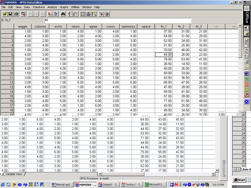
First, SPSS actually computes more than one additional column. In particular, the number of additional columns that SPSS computes equals the number of groups minus 1 or the number of dependent measures, whichever is smaller. Each column is designed to maximize the difference between groups, with one restriction. Specifically, each column must be uncorrelated with the previous columns. For example, in the table below, Functions 1, 2 and 3 are uncorrelated with one another. An understanding of Discriminant Function Analysis would provide a more comprehensive appreciation of these columns.

Another important complication needs to be appreciated. Several definitions can be applied to reflect the difference between the groups. To illustrate, SPSS could calculate:

• The average difference between each pair of averages on all the functions.
• The smallest different between any pair of averages on all the functions.

Indeed, SPSS could compute more complex indices, which are somewhat difficult to understand, such as:

• The variance of all these averages, sometimes called the Pillais trace.
• The variance of scores within groups, divided by the total variance, sometimes called Wilks Labmda.
• The variance of these averages, divided by the variance within groups, sometimes called Hotelling"s trace.
• The same as above, but for one function only, sometimes called Roy's Largest Root.

Accordingly, SPSS does not merely ascertain one formula that maximises the difference between groups. Instead, SPSS needs to derive a formula for each possible definition. For example, the formula:

• Function 1 = 2.5 x Extroversion + 1.5 x Neuroticism + 4.0 x Conscientiousness + 5.0 x Agreeableness + 4.5 x Openness to Experience

might maximise the variance of all these averages. In contrast, the formula:

• Function 1 = 6.3 x Extroversion + 0.7 x Neuroticism + 3.1 x Conscientiousness + 1.3 x Agreeableness + 5.2 x Openness to Experience

might maximize variance of these averages, divided by the variance within groups. In other words, SPSS actually creates many additional formulas to combine the measures. Each formula is intended to maximize the differences between the groups. However, each formula applies a different definition of maximum difference. The following table illustrates the various columns that SPSS creates. In other words, SPSS utilises four of the definitions that were presented earlier.

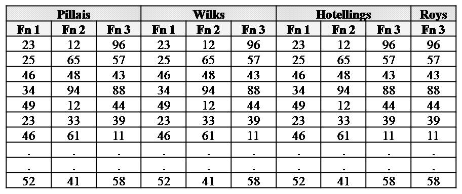
Using these additional columns, SPSS then computes a Pillais trace, Wilks lambda, Hotellings trace, and Roys LR, utilizing the complex definitions that were presented earlier. Additional formulas have been formulated to convert each index to an F and significance value. In other words, the information that is presented in the table called 'Multivariate tests' really derives from many complex operations.

The various indices--Pillais trace, Wilks lambda, Hotellings trace, and Roys LR--provide the same p values when the factor entails two groups only. When the factor entails more than two groups, these p values can diverge from one another. The researcher must decide which p value to utilise in advance.

• Many researchers utilise the Pillais trace, when the assumption of homogenous covariances is violated.
• Otherwise, they tend to use Wilks lambda, which is more powerful than Pillais trace in many situations.

To summarise, MANOVA combines all the measures into several columns that are intended to maximize the difference between groups. In reality, MANOVA undertakes this process on several occasions to reflect different formulas to measure this difference between groups.

Rationale behind two-way MANOVAs

The previous discussion focussed solely on one-way MANOVAs. An analogous rationale underpins two-way MANOVAs. The principal complication is that SPSS undertakes the process for each main effect and interaction separately. Specifically:

• SPSS creates additional columns that maximise the difference between the groups associated with one variable, such as favourite Wiggle, using the process that was delineated earlier.
• These columns are then analysed to ascertain whether or not the measures, personality, are significantly related to the first factor, favourite Wiggle.
• SPSS then creates another set of additional columns that maximise the difference between the groups associated with the other variable, such as favourite Osborne, using the same process.
• These columns are then analysed to ascertain whether or not the measures, personality, are significantly related to the second factor, favourite Osborrne.
• Finally, SPSS create another set of additional columns that maximise the interaction between the two factors, using an analogous process& in particular, these columns maximise the extent to which the difference between the groups associated with one factor vary across the levels of the other factor.
• Again, these columns are analysed to ascertain whether or not the interaction is significant.

STep 2: Examine the measures separately

Thus far, the researcher has been able to ascertain whether or not favourite Wiggle or Osborne is related to personality. If none of the main effects or interactions attain significance, the researcher would not proceed any further. They would conclude that no evidence exists that personality varies with favourite Wiggle or Osborne. Additional ANOVAs would be inappropriate, because the likelihood of Type I errors would be inflated beyond 0.05.

If the interaction is significant, however, the researcher would then subject each measure to a separate two-way ANOVA. This process ascertains which of the measures vary with the factors. Most researchers apply a Bonferroni adjustment to these ANOVAs. Nevertheless, you could argue these adjustments are unnecessary, because the ANOVAs do not yield overlapping conclusions. If a main effect is significant, but the interaction is not significant, a series of one-way ANOVAs would be more applicable. In particular:

• The researcher would apply each measure to a separate one-way ANOVA.
• The significant main effect in the MANOVA becomes the factor in the subsequent ANOVAs.

SPSS actually provides the output of these ANOVAs by default. However, many researchers prefer to undertake the ANOVAs themselves, because they can then dictate the analysis of simple effects and post-hoc tests.

Repeated measures MANOVA

The same fundamental rationale applies if one or more of the factors are repeated measures. The process to conduct repeated-measures MANOVAs, however, is marginally more complex. In other words, if the same participants are assessed in different conditions, a different process must be undertaken. To illustrate this technique, suppose instead that personality of individuals is measured after they watch one hour of each Wiggle. Hence, personality is assessed on four separate occasions. An extract of the data is provided below. The first letter of each variable denotes the Wiggle. For instance, 'm' refers to Murray. The remaining letters of each variable denote the personality measure. For example, 'extra' refers to extraversion.

To conduct the repeated-measures MANOVA:

1. Select "General Linear Model" and then "Repeated Measures" from the "Analyse" menu, after opening the relevant data file.
2. In the box labelled 'Within-subject factor name', create a name for your repeated measures factor, such as 'Wiggle'.
3. Specify the number of levels or categories associated with this factor, such as '4', and press 'Add'.
4. Press the button labelled 'Measures'.
5. In the box labelled 'Measures', specify the name of one of your measures, such as 'Openness'. Press Add and apply the same process to each measure.
6. Press Define.

This procedure activates the following dialogue box.

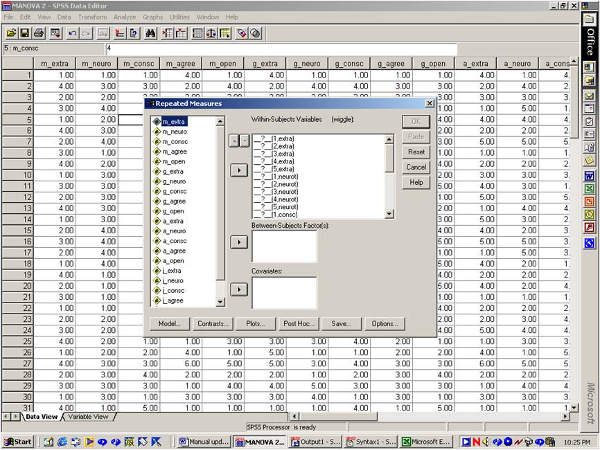
The left hand box displays all the column labels in the SPSS data file. You need to specify the column label that pertains to each question mark in the box labelled 'Within-subjects variables'. For example:

• The column label that pertains to (1, extra) is 'm_extra'. That is, the first category of the variable 'Wiggles' is Murray. The column that reflects extraversion scores for Murray is 'm_extra'
• The column label that pertains to (2, neuro) is g_neuro'. That is, the second category of the variable 'Wiggles' is Greg. The column that reflects the neuroticism scores for Greg is 'g_neuro', and so forth.

Once you have completed this process, you can also specify other between-subject factors, such as gender. Then press OK. The output should resemble the information that emerges for MANOVAs in which no repeated measures are included.

Illustration of the format used to report MANOVA

A MANOVA was undertaken to explore the effect of favourite Wiggle and favourite Osborne on personality, as gauged by the five factor model. The variance-covariance matrices were not homogenous, Box's M = .292, F(5, 132) = 6.75, p < .001, and hence the Pillais trace was utilised. Favourite Wiggle influenced personality, Pillais = 0.44, F(15, 138) = 1.59, p < .001. On the other hand, favourite Osborne did not influence personality, Pillais = .23, F(15, 138) = .77, p > .05. Likewise, favourite Osborne did not influence the effect of favourite Wiggle on personality, Pillais = .79, F(45, 240) = 1.21, p > .05.

Univariate one-way ANOVAs revealed that favourite Wiggle did indeed influence neuroticism, F(1, 132) = 9.56, p < .001 and extraversion, F(1, 132) = 8.76, p < .001, but did not affect the other personality scales. Table 1 presents the mean and standard deviation of neuroticism and extraversion as a function of favourite Wiggle. Finally, pairwise comparisons revealed that..."

Table 1. Mean neuroticism and extraversion as a function of favourite Wiggle. Standard deviations are presented in parentheses.